
Made By Yifeng Tang
GitHub Page
HW5
Background
The goal of this project is to train a deep learning model to classify beetles, cockroaches and dragonflies using these Images Sets. The images are from Here. Also, in the end, I used Shaply Explanations to evaluate the prediction result.
Strategy
I used Tensorflow, which is a powerful images classification tool. The procedure of this machine learning project is:
- Overview and understand the data
- Build an input pipepline
- Create the model
- Train the model
- Test the model
- Evaluate the model
Environment
The following are the required packages for this project:
import matplotlib.pyplot as plt
import numpy as np
import os
import PIL
import tensorflow as tf

from tensorflow import keras
from tensorflow.keras import layers
from tensorflow.keras.models import Sequential
import pathlib
import glob

import shap
The edition of the required packages are:
matplotlib == 3.3.1.
numpy == 1.19.1.
tensorflow == 2.7.0.
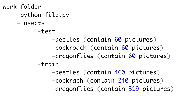
The following is the structure of the work directory for this project:
Preparing the data:
Overview:
There are total number of 1019 pictures for train data. In the 1019 pictures, there are 460 for beetles, 240 for cockroach, and 319 for dragonflies.
There are total number of 180 pictures for test data.
You could use the following code to achive this:
#train overall: number of total tarin pictures
train = [f for f in glob.glob('insects/train/*/*.jpg')]
print(len(train))

#test overall: number of total test pictures:
test = [f for f in glob.glob('insects/test/' + "*/*.jpg")]
print(len(test))

#train for beetles: number of train
train_beetles = [f for f in glob.glob('insects/train/beetles/*.jpg')]
print(len(train_beetles))
#number of train cockroach
train_cock = [f for f in glob.glob('insects/train/cockroach/*.jpg')]
print(len(train_cock))
#number of train dragonflies
train_drag = [f for f in glob.glob('insects/train/dragonflies/*.jpg')]
print(len(train_drag))
Standardized the images: Before using the training data to create the model, we need to standardize the pictures first:
#standardized the picture
batch_size = 32
img_height = 180
img_width = 180

#training data set:
train_ds = tf.keras.utils.image_dataset_from_directory(
  'insects/train/',
  image_size=(img_height, img_width),
  batch_size=batch_size)

#stabdardized test data set:
test_ds = tf.keras.utils.image_dataset_from_directory(
  'insects/test/',
  image_size=(img_height, img_width),
  batch_size=batch_size)

# keeps the images in memory after they're loaded off disk during the first epoch.
AUTOTUNE = tf.data.AUTOTUNE

train_ds = train_ds.cache().shuffle(1000).prefetch(buffer_size=AUTOTUNE)
test_ds = test_ds.cache().prefetch(buffer_size=AUTOTUNE)

# standardized the pictures
normalization_layer = layers.Rescaling(1./255)
normalized_ds = train_ds.map(lambda x, y: (normalization_layer(x), y))
image_batch, labels_batch = next(iter(normalized_ds))
first_image = image_batch[0]
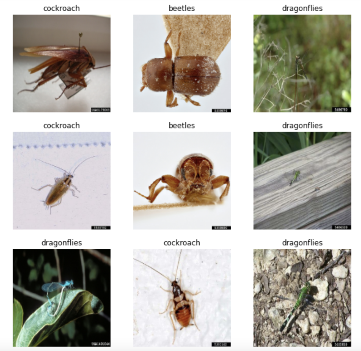
Let’s see some samples of the data:
Create the model:
The Sequential model consists of three convolution blocks (tf.keras.layers.Conv2D) with a max pooling layer (tf.keras.layers.MaxPooling2D) in each of them. There’s a fully-connected layer (tf.keras.layers.Dense) with 128 units on top of it that is activated by a ReLU activation function (‘relu’). This model has not been tuned for high accuracy—the goal of this tutorial is to show a standard approach.
# 3 types of insects
num_classes = 3

# create the model:
model = Sequential([
  layers.Rescaling(1./255, input_shape=(img_height, img_width, 3)),
  layers.Conv2D(16, 3, padding='same', activation='relu'),
  layers.MaxPooling2D(),
  layers.Conv2D(32, 3, padding='same', activation='relu'),
  layers.MaxPooling2D(),
  layers.Conv2D(64, 3, padding='same', activation='relu'),
  layers.MaxPooling2D(),
  layers.Flatten(),
  layers.Dense(128, activation='relu'),
  layers.Dense(num_classes)
])

# Compile the model
model.compile(optimizer='adam',loss=tf.keras.losses.SparseCategoricalCrossentropy(from_logits=True),
              metrics=['accuracy'])
Train the model
#Train the model
epochs=10
history = model.fit(
  train_ds,
  validation_data=test_ds,
  epochs=epochs
)
Prediction
Now, we have created our own model! We could use the model to do some simple predictions for those three insects.
By using the following code:
#prediction:
img = tf.keras.utils.load_img(
    'meme.jpg', target_size=(img_height, img_width)
) # change the 'meme.jpg' to your own image.
img_array = tf.keras.utils.img_to_array(img)
img_array = tf.expand_dims(img_array, 0) # Create a batch

predictions = model.predict(img_array)
score = tf.nn.softmax(predictions[0])

print(
    "This image most likely belongs to {} with a {:.2f} percent confidence."
    .format(class_names[np.argmax(score)], 100 * np.max(score))
)
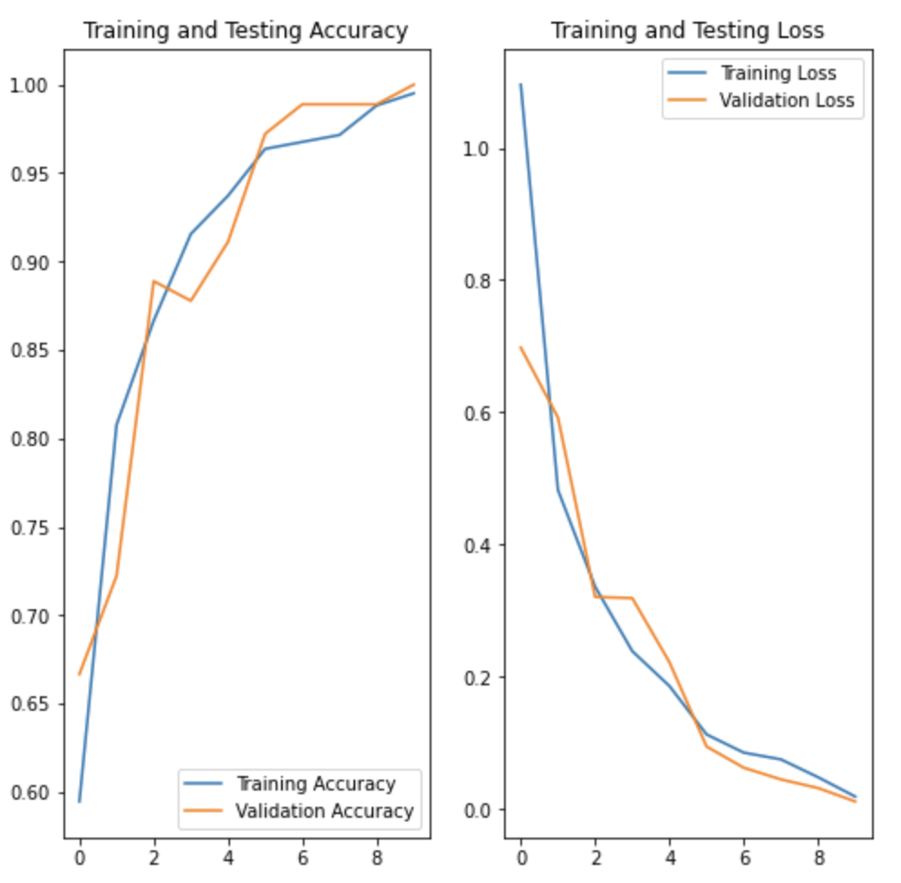
Visualizing the model performance
We could use the following code to create plots of loss and accuracy on the training and validation sets:
acc = history.history['accuracy']
val_acc = history.history['val_accuracy']

loss = history.history['loss']
val_loss = history.history['val_loss']

epochs_range = range(epochs)

plt.figure(figsize=(8, 8))
plt.subplot(1, 2, 1)
plt.plot(epochs_range, acc, label='Training Accuracy')
plt.plot(epochs_range, val_acc, label='Validation Accuracy')
plt.legend(loc='lower right')
plt.title('Training and Testing Accuracy')

plt.subplot(1, 2, 2)
plt.plot(epochs_range, loss, label='Training Loss')
plt.plot(epochs_range, val_loss, label='Validation Loss')
plt.legend(loc='upper right')
plt.title('Training and Testing Loss')
plt.show()
The plot is like:
SHAP Evaluation
SHAP (SHapley Additive exPlanations) is a game theoretic approach to explain the output of any machine learning model. It connects optimal credit allocation with local explanations using the classic Shapley values from game theory and their related extensions.
To get the shap value, we need some steps to do some preparation. The first is data prepared:
In order to use SHAP help us evaluate the model, we need to change the train data and test data to matrix format:
# convert the train data set to matrix form
x_train = np.concatenate([x for x, y in train_ds], axis = 0)
y_train = np.concatenate([y for x, y in train_ds], axis = 0)

# convert the test data set to matrix form
x_test = np.concatenate([x for x, y in test_ds], axis = 0)
y_test = np.concatenate([y for x, y in test_ds], axis = 0)
======.
Then we need to prepare some variables to compute SHAP value.
We use the DeepExplainer class from the shap librar to explain predictions of the model we just built.
explainer = shap.GradientExplainer(model, x_train)
Eventually, compute the SHAP value:
#calculate the shap value:
sv = explainer.shap_values(x_test[:20])
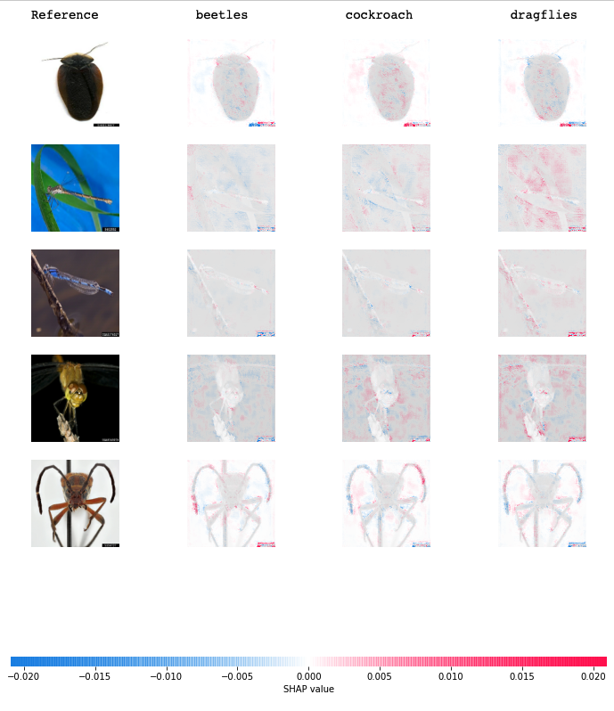
Visulization of the SHAP values
Sometimes, it is hard to understand the simple score of SHAP. Here, We could take a look at the computed shap values.
To understand the plot, here are some rules:
- Positive shape values are represented by red, and they represent pixels that help classify the image into that particular category.
- Negative shap values are denoted by blue color and they represent the pixels that contributed to NOT classify that image as that particular class.
- Each row contains each one of the test images you computed the shap values for. The example contains 3 classes.
print("    Reference             beetles             cockroach             dragflies")
shap.image_plot([sv[i] for i in range(3)], x_test[0:5])
Following is the sv image. The first row in reference is cockroach, we can observe there more red part in the imagine under the cockroach column.It indicates that the classification accuracy is satisfied.
====end